EnrichMap resolves opposing gene programmes#
This tutorial demonstrates how to use EnrichMap when the upregulated and downregulated gene programmes are known for the pathway of interest.
import os
os.environ["PYTHONWARNINGS"] = "ignore"
import warnings
warnings.filterwarnings("ignore")
Import required packages for minimal example.
import scanpy as sc
import enrichmap as em
sc.set_figure_params(frameon=False)
Read in the dataset:
adata = sc.read(
    "adata_breast.h5ad",
    backup_url="https://github.com/secrierlab/EnrichMap/raw/main/tests/dataset/adata_breast.h5ad",
)
As the data is shared as raw counts, we normalise them.
sc.pp.normalize_total(adata, target_sum=1e4)
sc.pp.log1p(adata)
Here, we investigate G0 arrest in breast cancer. The gene signature is taken from Wiecek et al (2023).
upregulated_genes = [
    "CFLAR", "CALCOCO1", "YPEL3", "CST3", "SERINC1", "CLIP4", "PCYOX1", "TMEM59",
    "RGS2", "YPEL5", "CD63", "KIAA1109", "CDH13", "GSN", "MR1", "CYB5R1", "AZGP1",
    "ZFYVE1", "DMXL1", "EPS8L2", "PTTG1IP", "MIR22HG", "PSAP", "GOLGA8B", "NEAT1",
    "TXNIP", "MTRNR2L12"
]

downregulated_genes = [
    "NCAPD2", "PTBP1", "MPHOSPH9", "NUCKS1", "TCOF1", "SART3", "SNRPA", "KIF22",
    "HSP90AA1", "WBP11", "CAD", "SF3B2", "KHSRP", "WDR76", "NUP188", "HSP90AB1",
    "HNRNPM", "SMARCB1", "PNN", "RBBP7", "NPRL3", "USP10", "SGTA", "MRPL4", "PSMD3",
    "KPNB1", "CBX1", "LRRC59", "TMEM97", "NSD2", "PRPF19", "PTGES3", "CPSF6", "SRSF3",
    "TCERG1", "SMC4", "EIF4G1", "ZNF142", "MSH6", "MRPL37", "SFPQ", "STMN1", "ARID1A",
    "PROSER1", "DDX39A", "EXOSC9", "USP22", "DEK", "DUT", "ILF3", "DNMT1", "NASP",
    "HMGB1P5", "SRRM1", "GNL2", "RNF138", "SRSF1", "TRA2B", "SMPD4", "ANP32B", "HMGA1",
    "MDC1", "HADH", "ARHGDIA", "PRCC", "HDGF", "SF3B4", "UBAP2L", "ILF2", "PARP1",
    "LBR", "CNOT9", "PPRC1", "SSRP1", "CCT5", "DLAT", "HNRNPU", "LARP1", "SCAF4",
    "RRP1B", "RRP1", "CHCHD4", "GMPS", "RFC4", "SLBP", "PSIP1", "HNRNPK", "SKA3",
    "DIS3L", "USP39", "GPS1", "PA2G4", "HCFC1", "SLC19A1", "ETV4", "RAD23A", "DCTPP1",
    "RCC1", "EWSR1", "ALYREF", "PTMA", "HMGB1", "POM121", "MCMBP", "TEAD4", "CHAMP1",
    "TOP1", "PRRC2A", "RBM14", "HMGB1P6", "POM121C", "UHRF1"
]
We first build directional gene weights using the upregulated_genes and downregulated_genes lists in the G0 programme. The build_signed_weights() function computes CV-based magnitudes and uses differential spatial correlation against the upregulated and downregulated reference patterns to assign signed weights.
directional_gene_weight_dict = em.tl.build_signed_weights(adata, up_genes=upregulated_genes, down_genes=downregulated_genes, score_key="enrichmap")
We now calculate EnrichMap scores for the G0 arrest programme. As there is more than one slide in this dataset, we specify the batch information stored in adata.obs. Note that when using weighted signatures, we use the gene_weights argument instead of gene_set.
em.tl.score(adata, gene_weights=directional_gene_weight_dict, batch_key="batch")
Scoring enrichmap: 126/126 genes found: 100%|██████████| 1/1 [00:02<00:00, 2.15s/it]
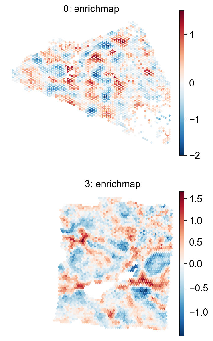
em.pl.spatial_enrichmap(
    adata,
    score_key=["enrichmap_score"],
    size=2,
    library_key="batch",
    library_id=["0", "3"],
    cmap="RdBu_r",
    shape=None
)
Evaluate spatial autocorrelation#
We can assess the spatial structure of the G0 arrest score using a Moran’s scatter plot.
em.pl.morans_correlogram(
    adata,
    score_key="enrichmap_score",
    library_key="batch",
    library_id=["0", "3"]
)
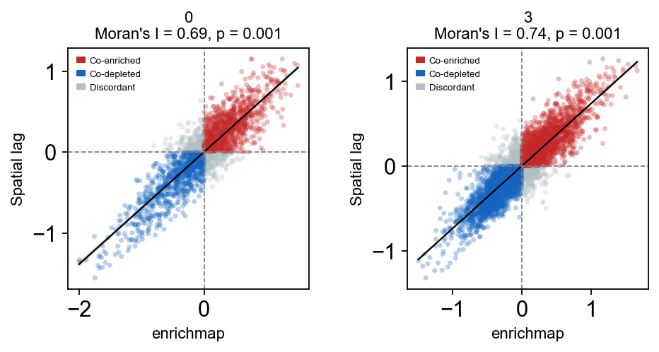
The Moran’s scatter plot confirms spatial autocorrelation of the signed G0 arrest score, with co-enriched and co-depleted spots clustering as expected.