EnrichMap tutorial for multiple samples

This tutorial demonstrates how to use EnrichMap with multiple slides. It is self-contained, but for a detailed introduction to single-signature scoring, spatial diagnostics and gene contribution analysis, see EnrichMap tutorial for one sample.

import os
os.environ["PYTHONWARNINGS"] = "ignore"

import warnings
warnings.filterwarnings("ignore")

Import required packages for minimal example.

import scanpy as sc
import squidpy as sq
import enrichmap as em

sc.set_figure_params(frameon=False)

Read in the dataset:

adata = sc.read(
    "adata_breast.h5ad",
    backup_url="https://github.com/secrierlab/EnrichMap/raw/main/tests/dataset/adata_breast.h5ad",
)

As the data is shared as raw counts, we normalise them.

sc.pp.normalize_total(adata, target_sum=1e4)
sc.pp.log1p(adata)

Scoring a single pathway across slides

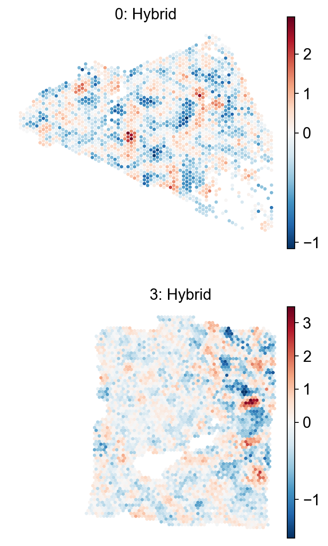
We start with a single signature to demonstrate multi-sample scoring. Here we score the hybrid EMT state across all slides. The key difference from single-sample usage is the batch_key argument, which ensures that batch normalisation, spatial smoothing and GAM correction are applied per slide.

The gene signature is taken from Malagoli Tagliazucchi et al. (2023).

Hybrid = ["PDPN", "ITGA5", "ITGA6", "TGFBI", "LAMC2", "MMP10", "LAMA3", "CDH13", "SERPINE1", "P4HA2", "TNC", "MMP1"]
Mesenchymal = ["VIM", "FOXC2", "SNAI1", "SNAI2", "TWIST1", "FN1", "ITGB6", "MMP2", "MMP3", "MMP9", "SOX10", "GCS", "ZEB1", "ZEB2", "TWIST2"]
Epithelial = ["CDH1", "DSP", "OCLN", "CRB3"]

em.tl.score(
    adata,
    gene_set=Hybrid,
    score_key="Hybrid",
    batch_key="batch"
)

Scoring Hybrid: 12/12 genes found: 100%|██████████| 1/1 [00:00<00:00,  1.91it/s]

em.pl.spatial_enrichmap(
    adata,
    score_key=["Hybrid_score"],
    size=2,
    library_key="batch",
    library_id=["0", "3"],
    cmap="RdBu_r",
    shape=None
)

Scoring multiple pathways across slides

When more than one signature is of interest, EnrichMap accepts a dictionary where each key is the signature name (used for storing scores in adata.obs) and the corresponding value is the gene list.

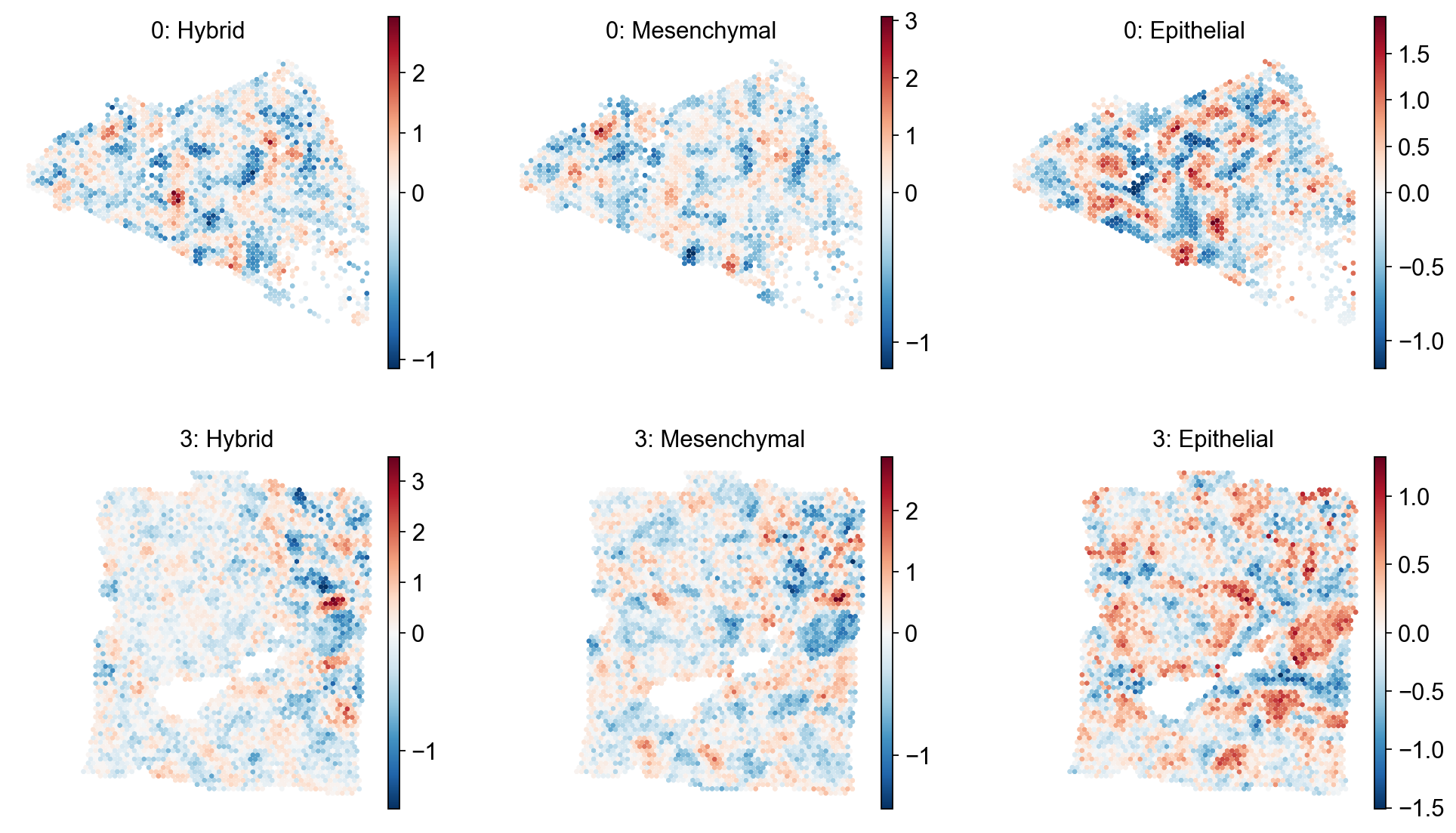
We now extend this to three EMT states: epithelial, hybrid and mesenchymal.

signature_dict = {
    "Hybrid": Hybrid,
    "Mesenchymal": Mesenchymal,
    "Epithelial": Epithelial
}

We now calculate EnrichMap scores for the three signatures. As there is more than one slide in this dataset, we specify the batch information stored in adata.obs.

em.tl.score(
    adata,
    gene_set=signature_dict,
    batch_key="batch"
)

Scoring Epithelial: 4/4 genes found: 100%|██████████| 3/3 [00:01<00:00,  2.57it/s]   

em.pl.spatial_enrichmap(
    adata,
    score_key=["Hybrid_score", "Mesenchymal_score", "Epithelial_score"],
    size=2,
    library_key="batch",
    library_id=["0", "3"],
    cmap="RdBu_r",
    shape=None
)

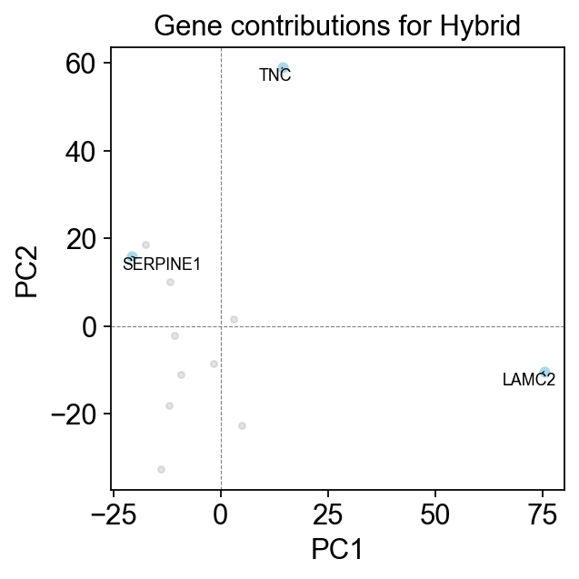
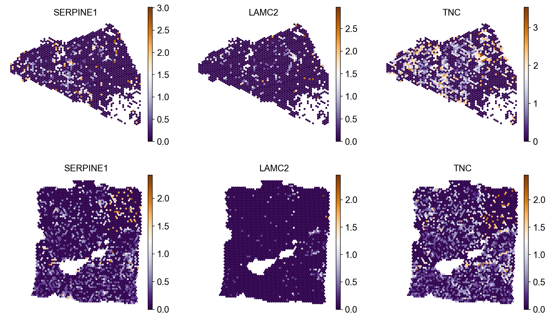
Let’s now investigate what genes influenced the hybrid state the most. Here, we demonstrate top three genes.

em.pl.gene_contributions_pca(
    adata,
    score_key="Hybrid_score",
    top_n_genes=3
)

Here’s the individual gene expression for top three genes.

sq.pl.spatial_scatter(
    adata,
    color=["SERPINE1", "LAMC2", "TNC"],
    library_key="batch",
    size=2,
    ncols=3,
    cmap="PuOr_r",
    shape=None
)

EnrichMap also implements a function to correlate multiple signatures to investigate co-acting biological pathways.

em.pl.signature_correlation_heatmap(
    adata,
    tile_size=0.5,
    score_keys=["Hybrid_score", "Mesenchymal_score", "Epithelial_score"],
)

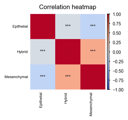
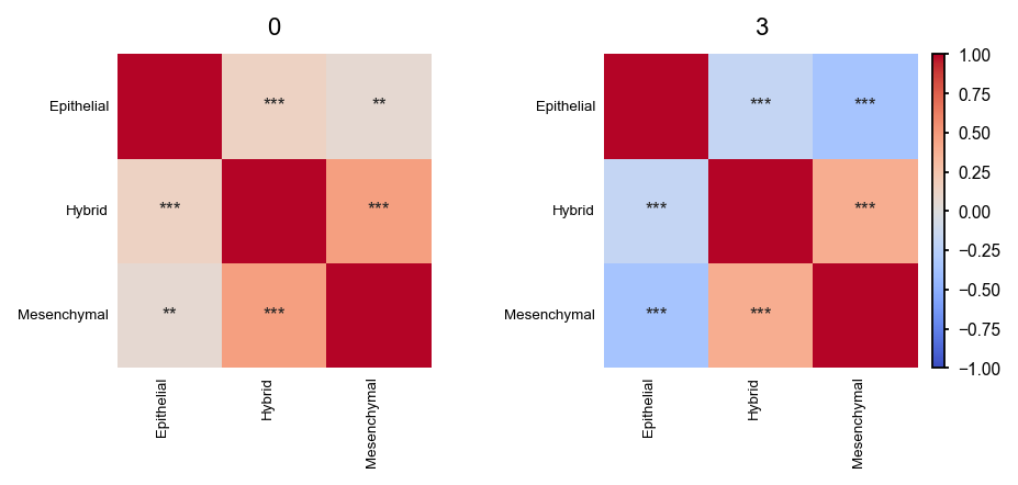
The heatmap above shows correlation between signatures across all slides. However, one might want to investigate this per slide.

em.pl.signature_correlation_heatmap(
    adata,
    score_keys=["Hybrid_score", "Mesenchymal_score", "Epithelial_score"],
    library_key="batch",
    tile_size=0.5,
)

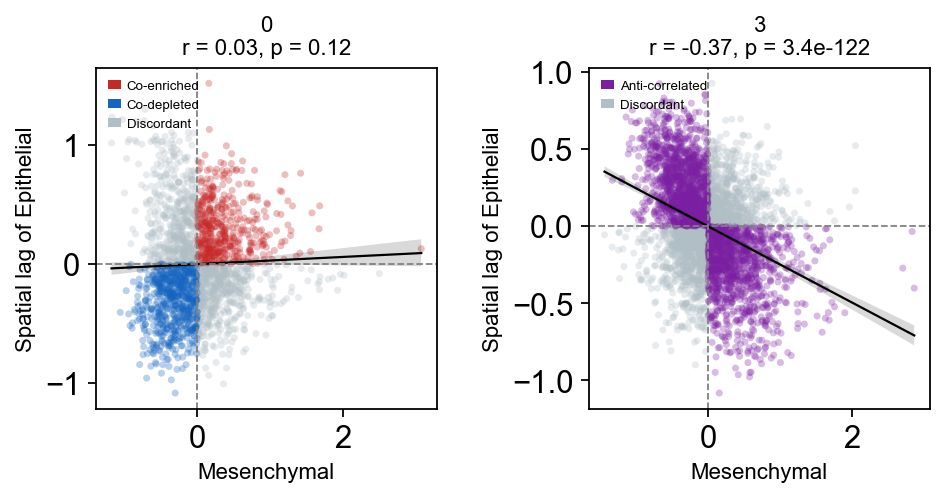
Cross-Moran analysis

Cross-Moran analysis assesses the spatial relationship between two scores by comparing one score against the spatial lag of the other. A positive correlation indicates that regions enriched for one programme are spatially surrounded by regions enriched for the other (co-localisation), while a negative correlation indicates spatial mutual exclusivity. Here, we test whether epithelial and mesenchymal programmes are spatially anti-correlated, as expected for reciprocal EMT states.

em.pl.cross_moran_scatter(
    adata, score_x="Mesenchymal_score", score_y="Epithelial_score", library_key="batch"
)

Comparing spatial scores across slides

When working with multiple samples, it is often useful to assess how similar or different the spatial enrichment patterns are between slides. EnrichMap provides two complementary approaches for this. The Wasserstein distance (also known as Earth Mover’s distance) quantifies how much “effort” is needed to transform one score distribution into another. Lower values indicate more similar distributions between slides.

em.pl.compare_wasserstein(
    adata, score_key="Mesenchymal_score", batch_key="batch", plot=False, figsize=(4, 4)
)

Wasserstein distances: 100%|██████████| 1/1 [00:00<00:00,  2.72it/s]

	0	3
0	0.000000	0.159255
3	0.159255	0.000000

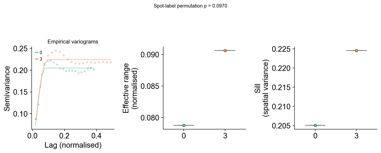
While the Wasserstein distance compares score distributions, variograms compare the spatial structure itself. By overlaying variograms from different slides, we can assess whether the spatial scale and strength of enrichment patterns are consistent across samples. Slides with similar variograms share similar spatial organisation, regardless of differences in absolute score values.

em.pl.compare_variograms(adata, score_key="Mesenchymal_score", batch_key="batch")

Fitting variograms: 100%|██████████| 2/2 [00:01<00:00,  1.58it/s]

	patient	effective_range	sill	nugget	nugget_sill_ratio
0	0	0.078765	0.205078	0	0.0
1	3	0.090646	0.224567	0	0.0